Prometheus 101
Take the “red pill” and let’s dive into monitoring basics with Prometheus.

Post structure:
- KEEP IT SIMPLE
- COUNTERS
- rate() vs irate()
- CPU usage
- Setup
Keep It Simple
source: https://www.robustperception.io/keep-it-simple-scrape_interval-id
spoiler:
- Keep things simple.
- Pick one scrape interval, and stick with it.
- Preferably not just per Prometheus, but across your team/organisation.
- A value in the range of 10-60s tends to be good.
🤔 Q: How many scrape intervals should I have in Prometheus?
In the Prometheus configuration there are two places you can configure the scrape interval: a default in the *global* section and then per-*scrape_config* overrides.
So you could decide that normally you want to scrape everything
every 10s, but there’s some key servers that you would like 2s for, and
other key ones that are a little slower so maybe 4s is the right
setting. Then there’s a really slow exporter that needs 1m, and an even
slower one that needs 3m. So sounds like 2s, 4s, 10s, 1m and 3m is the
way to go!
Please don’t.
- The first issue is the complexity of this configuration. Every time a new service is added you need to spend time figuring out which category it falls under, and maybe even add a new value.
- Secondly once the data is in the Prometheus, when writing queries you usually need to know the interval of the underlying data so that you can choose the most appropriate range for your
rate(). The more intervals you have, the more likely that you’ll not get that quite right. In addition working with data with different intervals can be a little tricky, as for examplerate()s with different ranges are not comparable.
🤔 Q: Can I use single-digit seconds interval?
Intervals on the order of single-digit seconds is getting into profiling territory. While a metrics-based system like Prometheus can handle that in certain cases, Prometheus is not a general profiling tool and thus not the most appropriate for the job. Profiling with Prometheus takes some care in design, and is not something you always want to mix in with your general monitoring.
🤔 Q: But… I need higher resolution!
For some problems metrics will not suffice and you will need to incorporate logs, tracing and/or profiling into your debugging. The more instrumentation you have in your code, the easier is to debug as the additional metrics will help you narrow down and correlate issues. For the problems where resolution does matter (e.g. microbursts) it is not guaranteed that metrics will be able to capture the issue, whereas logs should always spot it**.** Metrics are complementary to other types of monitoring and debugging tools, not a replacement. Metrics give you a good view of how things are working at the system and subsystem levels, but don’t cover individual requests or instruction-level timings.
Counters
sources: https://www.robustperception.io/how-does-a-prometheus-counter-work
There are four standard types of metric in Prometheus instrumentation:
- Gauge,
- Counter,
- Summary and
- Histogram
Counters: the problem & the approach
Example: How does one “count” the requests a system gets per second? There are three common approaches.
- The first is that on a regular basis, such as once a minute, you extract the current value which goes to you monitoring system, and reset the counter to 0. This has a problem in that if the push fails, then you lose all information about that time period. This could leave you blind to a micro burst of traffic. Additionally, if you’ve two systems pulling data from the counter for redundancy, each will only see about half the increments. That’s not great.
- The second approach is to use some form of Moving Average, usually exponential. This means that recent data points have more importance than older data points. Depending on the phase and frequency of the increment pattern, relative to when the monitoring system samples information, you will get different results as not all data points are equal. This approach can handle multiple systems taking samples, but will lose information if a sample fails to be taken. This is better, but far from perfect.
- Prometheus takes the third approach. A counter starts at 0, and is incremented. The client does no other calculations. At each scrape Prometheus takes a sample of this state. The
rate()function in Prometheus looks at the history of time series over a time period, and calculates how fast it’s increasing per second. This can handle multiple Prometheus servers taking samples, and if a scrape fails you’ll lose resolution but not data as on the next successful scrape the increments haven’t been lost or averaged away.
Example: “receive_bytes” counter & iperf
I start with node_network_receive_bytes_total{device="eno1"} where {device="eno1"} is used to filter the many metrics received for different devices and continue by adding irate() to get the actual graph irate(node_network_receive_bytes_total{device="eno1"}[1m]). The 2 spikes shown were caused by 2 iperf tests (default settings 10sec-test).
# 1st iperf
- - - - - - - - - - - - - - - - - - - - - - - - -
[ ID] Interval           Transfer     Bandwidth
[  4]   0.00-10.00  sec   202 MBytes   169 Mbits/sec                  sender
[  4]   0.00-10.00  sec   202 MBytes   169 Mbits/sec                  receiver

# 2nd iperf
[ ID] Interval           Transfer     Bandwidth
[  4]   0.00-10.00  sec   912 MBytes   765 Mbits/sec                  sender
[  4]   0.00-10.00  sec   912 MBytes   765 Mbits/sec                  receiver
click to zoom 🔎
The basic idea:
- a counter is a metric that keeps increasing
- rate() calculates a per-second rate for a counter metric

Rate() vs irate()
source: https://www.robustperception.io/irate-graphs-are-better-graphs
irate graphs are better graphs
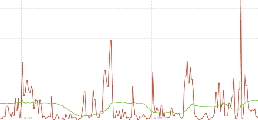
The rate function takes a time series over a time range,
and based on the first and last data points within that range (allowing
for counter resets) calculates a per-second rate. As it’s based on the
whole range, it’s effectively an average rate over that range – 5
minutes in this case. You can see that the green line in the graph above
is slow to pick up on changes, and not showing the full detail.
By contrast irate is an instant rate. It only looks at the last two points within the range passed to it and calculates a per-second rate. In the graph above the scrape interval is 10 seconds, so the red line is allowing you to see much briefer spikes and finer detail. This gives you better insight into what’s really going on, taking advantage of the full resolution of the data available.
Example: “receive_bytes” counter & iperf
Notice the wrong per-second rate calculated in the rate() case (it shows bytes being received for a whole minute! whereas iperf run for only 10 seconds!).
click to zoom 🔎

🤔 Q: What happens when the process restarts and the counter is reset to 0 (zero)?
rate() will automatically handle this. Any time a counter appears to decrease it’ll be treated as though there was a reset to 0 right after the first data point. This makes it important that it not be possible for Counters to be decremented, a Counter that has the potential to be decremented is in reality a Gauge.
🤔 Q: What happens when scrapping fails?
As with rate, irate is resilient to scrapes failing as it’ll look back to the previous successful scrape. This loses a little resolution, but you don’t miss any sudden changes around that failed scrape. This is one advantage of exporting raw counters over rates computed on the instrumented system.
🤔 Q: Which one should I use for alerting?
Due to the instant rate being more responsive, there are a few things you should be aware of. If you’re doing alerting based on irate a very brief dip could reset the alert’s FOR clause, so prefer rate for alerting. In graphs over long time periods used for trending, full resolution data can be distracting so the implicit averaging of rate is more useful.
CPU usage
from: Understanding Machine CPU usage
Our starting point is a metric exposed by the node-exporter named node_cpu_seconds_total which is of type counter.
This metric comes from /proc/stat and tells us how many seconds each CPU spent doing each type of work:
- user: The time spent in userland
- system: The time spent in the kernel
- iowait: Time spent waiting for I/O
- idle: Time the CPU had nothing to do
- irq&softirq: Time servicing interrupts
- guest: If you are running VMs, the CPU they use
- steal: If you are a VM, time other VMs “stole” from your CPUs
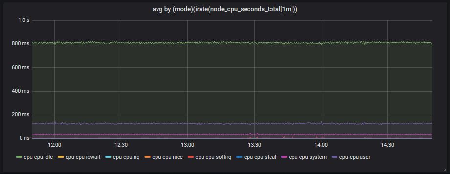
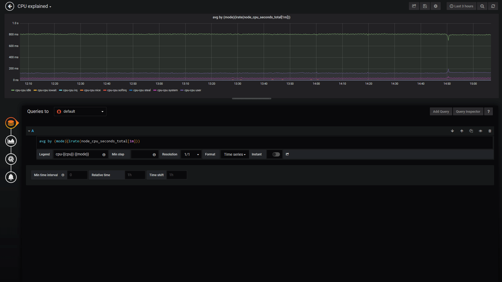
Notice that there are 8 different types of “CPU-work” counters. k8s-node (the machine used) has an i7 with 8 CPUs, so this means that we will have to calculate the CPU usage by doing some basic math on: 8CPUs x 8types = 64 values
The node has been up for about 4 days, that’s why the time counters (on the left) have reached day levels (especially the idle ones). If we use irate() to calculate the per-second time used (on the right) the results are within the 1 second.
- left picture :
node_cpu_seconds_total - right picture:
irate(node_cpu_seconds_total[1m])

It’s time to use sum()
To treat the different values coming from the 8 different CPUs as one single value, we can use sum().
And because this will end up to values summing up to 8 seconds, we
divide it by 8 (the number of CPUs) to make them sum up to 1 second.
- left picture :
sum by (mode)(irate(node_cpu_seconds_total[1m])) - right picture:
sum by (mode)(irate(node_cpu_seconds_total[1m])) / 8

With avg() it’s more dynamic…
What happens if a machine has 2, 4… etc CPUs? To make the above more
dynamic (as it is now you have to hard-code the CPU number) we can just
use avg() and result to the same graph.
avg by (mode)(irate(node_cpu_seconds_total[1m]))
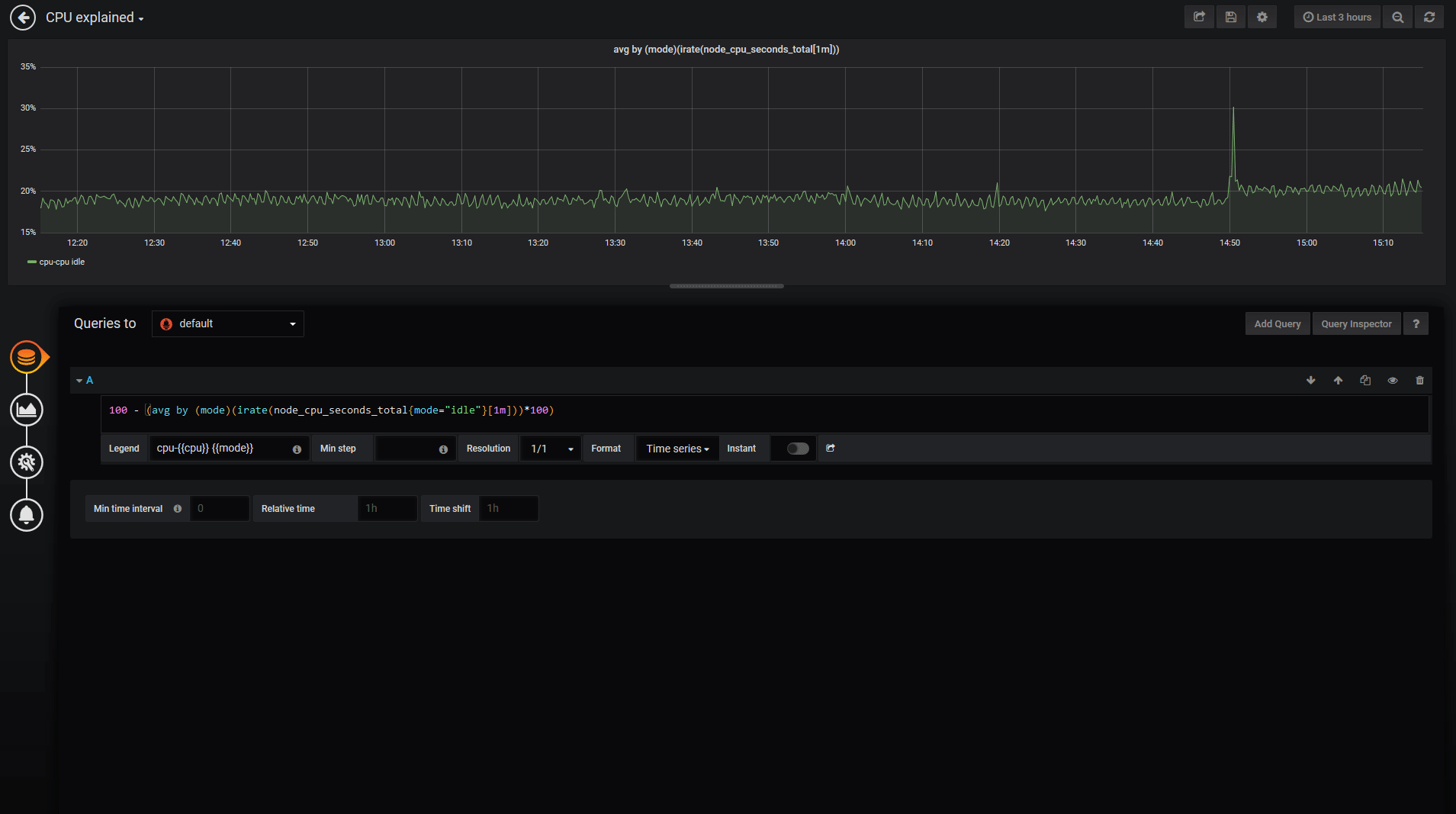
Calculate CPU usage %
We will use the following logic:
CPU usage = 100 - (idle_time*100) which means that we consider CPU usage everything except the idle time. The prometheus query now becomes:
100 - (avg by (mode)(irate(node_cpu_seconds_total{mode="idle"}[1m]))*100)
and at the end we also change the graph settings from seconds to percentage.
click to zoom 🔎
CPU usage Gauge
The same query can be used to show a gauge by changing the graph type and a few parameters. Notice, that “gauge” here doesn’t mean the gauge metric type of prometheus. Our metric is still a counter, we just use some graphana settings to show the current (latest) values and ignore the rest of them.
Command used to generate CPU spikes: stress --cpu 8 --timeout 20
Another useful CPU usage graph
In the previous steps we show everything apart from idle (100%-idle)
but sometimes we need to see what takes most of the CPU usage. Is it the
system, is it the user, is it an iowait
which might indicate a disk/network problem? On the left side is what
we have already used and on the right a slight modification (values sum
up to 1 second):
(avg(irate(node_cpu_seconds_total {mode!="idle"} [1m])) without (cpu))
Setup used: Medianetlab K8S cluster
k8s-master will run:
- a prometheus server to collect the data
- a grafana to create dashboards
Docker compose file 👇:
# docker-compose.yml

version: '3'

services:

  prometheus_srv:
    image: prom/prometheus
    container_name: prometheus_server
    hostname: prometheus_server
    restart: always
    volumes:
      - .:/etc/prometheus
    ports:
      - 9090:9090

  grafana:
    image: grafana/grafana
    container_name: grafana
    hostname: grafana
    restart: always
    user: "1000"
    volumes:
      - ./grafana_data:/var/lib/grafana
    depends_on:
      - prometheus_srv
    ports:
      - 3000:3000
scrapping:
- prometheus server itself at
k8s-master-IP:9090/metrics - grafana metrics at
k8s-master-IP/metrics - prometheus node at
k8s-node:9100/metrics - container metrics at
k8s-node:8080
Prometheus yaml file 👇:
# prometheus.yml

# my global config
global:
  scrape_interval:     10s # By default, scrape targets every 10 seconds.
  evaluation_interval: 10s # By default, scrape targets every 10 seconds.

scrape_configs:
  # Scrape Prometheus itself (k8s-master)
  - job_name: 'prometheus'
    scrape_interval: 10s
    scrape_timeout: 10s
    static_configs:
      - targets: ['localhost:9090']

# Scrape Prometheus (k8s-node)
  - job_name: 'k8s-node'
    scrape_interval: 10s
    scrape_timeout: 10s
    static_configs:
      - targets: ['k8s-node-IP:9100']

 # Scrape Grafana metrics
  - job_name: 'grafana'
    scrape_interval: 10s
    scrape_timeout: 10s
    static_configs:
      - targets: ['k8s-master-IP:3000']

# Scrape cAdvisor metrics (k8s-node)
  - job_name: cadvisor
    scrape_interval: 10s
    static_configs:
      - targets: [k8s-node-IP:8080]
k8s-node will run:
- a prometheus node-exporter to expose host metrics
- a cAdvisor to expose container metrics
Commands used to run the containers 👇:
#node_exporter

sudo docker run -d \
  --net="host" \
  --pid="host" \
  -v "/:/host:ro,rslave" \
  quay.io/prometheus/node-exporter \
  --path.rootfs /host


# cAdvisor
sudo docker run \
  --volume=/:/rootfs:ro \
  --volume=/var/run:/var/run:ro \
  --volume=/sys:/sys:ro \
  --volume=/var/lib/docker/:/var/lib/docker:ro \
  --volume=/dev/disk/:/dev/disk:ro \
  --publish=8080:8080 \
  --detach=true \
  --name=cadvisor \
  google/cadvisor:latest